Backends

Purpose

The open-source (Tier A) codes the Tokamak Toolkit drives, and exactly how their data is translated. Each translation is checked against a quantity the other code computes independently, because unit and grid mismatches produce plausible-looking plots.

TORAX: whole-code transport

TORAX (Google DeepMind, Apache-2.0) is a tokamak core transport simulator written in JAX: current diffusion, heat and particle transport, bootstrap current, fusion power, radiation, pedestal and sawtooth models, with QLKNN as its neural turbulent-transport model. The Tokamak Toolkit uses it in two ways: as a whole-code backend (TORAX’s own driver and adaptive time stepping, to produce references), and as the physics inside the Tokamak Toolkit’s fixed-step loop (see coupling loop).

Running a scenario

A scenario is one of TORAX’s example configurations (a Python CONFIG dict), with overrides deep-merged in (e.g. a shorter end time). The run is host-side, outside the Tokamak Toolkit’s compiled code, and returns TORAX’s output tree. Benchmarks in use: iterhybrid_rampup (80 s current ramp-up, QLKNN transport, Newton solver) and iterhybrid_predictor_corrector (5 s flat-top, the quicker check).

Translating the output

quantity	TORAX	Tokamak Toolkit	conversion
temperatures	keV	eV	× 1000
profile arrays	face 0, \(n\) cells, face \(n\)	\(n\) cells	drop the two boundary points
geometric factor	g1 \(=\langle\lvert\nabla V\rvert^2\rangle\)	\(G = \langle\lvert\nabla\rho\rvert^2\rangle\)	\(G = g_1 / V'^2\)
\(V'\)	vpr	vprime	none (\(\partial V/\partial\rho\) in both)
safety factor	on faces	on cells	linear interpolation
heat diffusivity	turbulent + neoclassical	chi_e, chi_i	sum
particle pinch	turbulent + neoclassical + Ware	v_e	sum
heating	one array per source and species	q_e, q_i	sum of p_*_e and p_*_i, then electron-ion exchange moved from electrons to ions
particle source	one array per source	s_n	sum of s_*

Checked by recomputing two quantities TORAX reports independently, from the converted data, at every output time:

• Total heating power, \(\sum_i (q_{e,i} + q_{i,i})\,V'_i\,\Delta\rho_i\) against TORAX’s P_heat_total: better than 10⁻⁸C-010.
• Stored thermal energy against TORAX’s W_thermal_total: 10⁻¹⁶C-009. This first came out 0.3% low, consistently. Not a conversion bug: ITER scenarios include a neon impurity (to radiate power before it reaches the wall) whose pressure contributes to the stored energy. Including impurity pressure closed the gap to round-off. A discrepancy of that size is easy to wave away, and would otherwise have been absorbed into “surrogate error” later.

Reference runs

Both benchmark scenarios are stored as TORAX output files with a provenance record beside each (scenario, TORAX version, full resolved config, commit), and both reproduce bit for bit when re-run. The 80 s ramp-up takes under 4 sC-023 once compiled on one datacentre GPU.

For ITER, the toroidal-flux radius at the boundary and the geometric minor radius differ by a factor of 1.37C-030; see K-007 on the IMAS adapters page for why that matters when exporting.

Energy and particle balance of a step

Purpose. M1’s acceptance asks that energy and particles are conserved to a tolerance on the benchmark. The toy model’s balance is checked in the transport solver tests; this is the same check for TORAX’s own discretisation.

Method. For each evolving channel \(x\) (ion and electron temperature, electron density, poloidal flux), TORAX’s finite-volume step with \(\theta = 1\) solves, on every cell,

\[ c_\text{out}^{\,n+1}\,\frac{c_\text{in}^{\,n+1} x^{n+1} - c_\text{in}^{\,n} x^{n}}{\Delta t} = \big(C\,x + c\big)^{n+1}, \]

where \(c_\text{out}, c_\text{in}\) are TORAX’s transient coefficients (for temperature, \(c_\text{out} c_\text{in} = \tfrac32 n V'\) in J/keV, written in the form \(V'^{-2/3}\partial_t(V'^{5/3} n T)\) that accounts for a changing geometry) and \(C x + c\) collects diffusion, convection and sources at the new time. Multiplying by the cell width \(\Delta\rho_i\) and summing over cells turns the equation into a global balance, because the diffusion and convection terms telescope to the flux through the last face (the face on the magnetic axis carries none):

\[ \underbrace{\textstyle\sum_i \Delta\rho_i\,\text{LHS}_i}_\text{storage} = \underbrace{\text{edge}}_{-\text{flux out}} + \text{sources} + \text{pinning} + \text{residual}. \]

Units are W for energy (\(T_i\) and \(T_e\) summed, so electron-ion exchange cancels) and electrons per second for particles.

Algorithm. Given the states before and after a step:

1. Rebuild the step’s inputs with TORAX’s own code: pre-step processing at \(t\) (explicit sources, pedestal state), runtime parameters and geometry at \(t + \Delta t\), the boundary-condition update.
2. Evaluate TORAX’s coefficients at the accepted new state, and at the old state for the transient term.
3. Assemble \(C x + c\) three times: complete; with the pedestal’s adaptive source switched off (its prefactors set to zero); and with every source term removed. The differences give pinning and sources; the last gives edge.
4. residual = storage − (edge + sources + pinning).

Nothing re-implements TORAX’s physics: every coefficient comes from TORAX. The residual is zero exactly when the accepted state satisfies TORAX’s own discrete equation. Steps on which a sawtooth crash replaced the equation solve are flagged and not balanced (none occurred in the runs below).

The pinning term. TORAX’s set_T_ped_n_ped pedestal model holds the temperatures and density at the pedestal top (\(\rho = 0.9\)) at prescribed values. It does so by adding a very large source \(k\,(x_\text{ped} - x)\) on that cell (TORAX’s default \(k\) is \(2\times10^{10}\) for temperature and \(2\times10^{8}\) for density): a numerical device, not a heating system. It injects or removes whatever power is needed to keep the pedestal where it is told to be. TORAX’s reported heating power does not include it, and the power it reports crossing the edge is heating minus \(\mathrm{d}W/\mathrm{d}t\), which therefore includes it.

Correctness.

• The edge term equals \(D\,\partial x/\partial\rho\) at the last face, computed separately from the face gradient: 10^-10C-039.
• Benchmark settings (ramp-up, Newton solver, 2 s steps): energy balance closes to better than 10^-6C-035 per step; particles to better than 10^-10C-036.
• The flat-top benchmark’s own solver (linear, one predictor-corrector step, Pereverzev terms) leaves about 0.8%C-037 of the energy balance unaccounted for. The global sum is insensitive to the Pereverzev terms, which telescope like any other transport term. What does not cancel is the lag in the coefficients the solver froze one iterate earlier: the fusion, radiation, ohmic and exchange sources, and the diffusivity at the edge face. More corrector steps shrink it, so it is the solver’s convergence, not the discretisation. Particles close to round-off with either solver: their sources in these scenarios do not depend on the state.

What the balance shows about the ramp-up. At every step after the first, the pedestal pinning source removes almost all of the heating power, and conduction through the edge carries only a small fraction (87–98%C-038). In this model, the heat that crosses the pedestal top leaves through the pinning source. Physically, that heat would flow through the pedestal and out. Conclusions about power crossing the edge (for example, L-H threshold margins) should be read with that in mind. It matters again at M5, where a discrepancy budget has to put the pinning power somewhere.

Design decisions.

• Rebuilt from TORAX, not re-derived. A second implementation of TORAX’s coefficients would test our copy, not TORAX. The one quantity computed independently is the edge flux (C-039), because it is the step on which the balance leans.
• Relative residual is |residual| divided by the sum of the magnitudes of the four terms, so a step with nearly cancelling large terms (the ramp-up) is not judged against a small net storage.

The RAPTOR L-mode benchmark

Purpose. M1’s first acceptance criterion is a match to published profiles. The one quantitative cross-code comparison published for TORAX is section V of the TORAX paper (Citrin et al., arXiv:2406.06718v4, CC BY 4.0): TORAX against RAPTOR on an ITER-like L-mode, with the configuration in Table II and the profiles in Fig. 6. It is the M1 physics benchmark (OQ-12). The ITER hybrid runs stay as the stiff-transport (QLKNN, Newton) and pedestal case.

Case. Constant \(I_p\) = 11.5 MA; 50 MW Gaussian heating centred at \(\hat\rho\) = 0.11, width 0.2, split equally between ions and electrons; constant transport \(\chi_i\) = 2, \(\chi_e\) = 1 m²/s, \(D_e\) = 1 m²/s, \(V_e\) = -0.15 m/s; Gaussian particle source 3 x 10²¹ /s at 0.2; Ohmic, fusion, ion-electron exchange and Sauter bootstrap current; no pedestal; CHEASE ITER hybrid equilibrium and its \(\psi\) as the initial condition; 50 cells; 10 s in fixed steps of 0.05 s; Newton-Raphson with 5 predictor-corrector steps. Table II uses an early TORAX’s parameter names; tkit/benchmarks/raptor_lmode/torax_config.py lists the translation line by line. Two points needed a choice:

• Impurity charge. Table II fixes \(Z_\text{imp}\) = 10. TORAX 1.4 computes neon’s charge from \(T_e\) (8.1 at the edge) unless it is overridden. With the computed charge, \(n_i\) differs from the paper’s TORAX curve by 0.35% with the computed charge, 0.009% with Z = 10C-056. The config fixes it at 10.
• Defaults not in Table II (implicit \(\theta\) = 1, no Pereverzev terms, Sauter conductivity) are TORAX 1.4’s. Where these changed between versions, the difference lands in the version line of the budget below.

Reference curves. Fig. 6 is vector graphics: each curve is a polyline whose vertices are the plotted points (51 for RAPTOR, 50 cell centres for TORAX, 51 faces for TORAX’s \(q\)). scripts/extract_raptor_fig6.py (pdfminer.six) reads every red (RAPTOR) and blue (TORAX) polyline inside each panel’s axes, names it from the legend entry with the same colour and dash pattern, and maps page to data coordinates with a least-squares line through the panel’s labelled tick marks. The largest tick residual is 6 x 10^-5 of an axis range. The curves are stored with the PDF’s sha256 in fig6_curves.json.

Error measure. The paper’s eq. (41), in percent:

\[ \text{NRMSD} = 100\,\frac{\sqrt{\tfrac{1}{N}\sum_i \big(y_i - y^\text{ref}(x_i)\big)^2}}{\tfrac{1}{N}\sum_i y_i} \]

over the compared run’s own points \(x_i\), with the reference interpolated linearly onto them. Recomputing it between the paper’s two curves returns each printed value (all five printed values reproduced (1.102, 0.712, 0.026, 0.414, 0.701% vs 1.1, 0.71, 0.03, 0.41, 0.70%)C-048). This checks the extraction and the convention together.

Results at t = 10 s, dt = 0.05 s (python -m tkit.cli benchmark-raptor --dt 0.05):

quantity	Tokamak Toolkit vs RAPTOR	Tokamak Toolkit vs paper’s TORAX	paper’s TORAX vs RAPTOR	printed in Fig. 6
\(T_i\)	1.23%	0.13%	1.10%	1.1%
\(T_e\)	0.28%	0.50%	0.71%	0.71%
\(n_e\)	0.031%	0.009%	0.026%	0.03%
\(n_i\)	0.031%	0.009%	0.026%
\(\psi\)	0.49%	0.08%	0.41%	0.41%
\(q\)	0.69%	0.16%	0.70%	0.70%
\(P_\text{fus,i}\)	21.5%	0.6%	22.0%
\(P_\text{fus,e}\)	13.3%	0.09%	13.3%
\(P_\text{ohm}\)	5.1%	3.6%	2.4%

The fusion-power split differs from RAPTOR by 13-22% in both TORAX versions alike; the paper attributes this to the codes’ different formulas for the fraction of alpha power going to ions. The largest change between TORAX versions is in \(P_\text{ohm}\) and \(T_e\) on axis (+1.4% → +0.5% against RAPTOR), both set by the parallel conductivity.

Time traces (line averages, maximum relative deviation over 0-10 s, and at 10 s):

trace	vs RAPTOR, max (time)	vs RAPTOR at 10 s	vs paper’s TORAX, max
\(\langle T_e \rangle\)	2.3% (2.3 s)	0.07%	0.42%
\(\langle T_i \rangle\)	2.4% (0.2 s)	1.0%	0.14%
\(\langle n_e \rangle\)	3.7% (0 s)	0.01%	0.19%

The paper reports a maximum transient deviation of about 2.5% between its codes’ temperature profiles. The 3.7% in density is the initial condition: RAPTOR’s average starts at 0.77, both TORAX runs at the requested 0.80 x 10²⁰ m^-3.

Time-step convergence. The same case at dt = 0.05, 0.025, 0.0125 and 0.00625 s (every step converged; the loop matches TORAX’s driver to 10^-13 at each):

	0.05 s	0.025 s	0.0125 s	0.00625 s
\(T_i\) vs RAPTOR, t = 10 s	1.2256%	1.2262%	1.2266%	1.2267%
\(\psi\) vs RAPTOR, t = 10 s	0.4886%	0.4865%	0.4855%	0.4850%
\(q\) vs RAPTOR, t = 10 s	0.6879%	0.6849%	0.6835%	0.6827%
\(\langle T_i \rangle\) vs RAPTOR, max over 0-10 s	2.40%	2.68%	2.84%	2.92%
\(\langle T_i \rangle\) vs paper’s TORAX, max	0.14%	0.49%	0.62%	0.69%

The end state is converged at the published step (at most 0.006 percentage pointsC-052). The transient is not: at dt → 0 the early ion temperature moves further from both published curves, which were made at 0.05 s. This is the time-discretisation line of the budget, reported separately as OQ-5 asks.

Acceptance tolerance (set at the M1 physicist review, 1 Oct 2026). Against RAPTOR: NRMSD of the t = 10 s profiles at most 2% for \(T_i\), \(T_e\), \(\psi\) and \(q\), and at most 0.1% for \(n_e\) and \(n_i\); the line-averaged traces within 5% of RAPTOR’s over 0-10 s. \(P_\text{fus,i}\), \(P_\text{fus,e}\) and \(P_\text{ohm}\) are reported, not gated. Every gated quantity passes at the published step and at 0.00625 s. The limits are ACCEPTANCE in tkit.physics.raptor_benchmark, checked by test_published_settings_pass_the_m1_acceptance_gate and printed by tkit.cli benchmark-raptor.

Discrepancy budget at t = 10 s (NRMSD, percent; what each line isolates):

line	size	how measured
wrapper: the Tokamak Toolkit’s loop vs TORAX’s driver	< 10-11	same config, same dt (better than 10-13C-049)
reading the figure	< 0.01	printed NRMSD recovered to its last digit
time discretisation (0.05 s → 0.00625 s)	≤ 0.006	dt series above
TORAX version and config translation	≤ 0.5 (\(T_e\)); 3.6 (\(P_\text{ohm}\))	vs the paper’s TORAX curves
physics and numerics, TORAX vs RAPTOR	0.03-1.2 (profiles); 13-22 (alpha split)	the paper’s TORAX vs RAPTOR

Other criteria on this case. Every step’s energy and particle balance closes (energy 1.1 × 10^-7, particles 3 × 10^-13C-054; method in the balance section). Reverse-mode gradients through Newton steps match central differences (6 × 10^-9C-055). TORAX 1.4.3 solves each Newton step inside jax.lax.custom_root, so both modes differentiate the converged solution implicitly. Forward mode first returned NaN in every tangent (ceiling K-009, now lifted): the rule’s explicit zero tangents for the geometry met TORAX’s \(\sqrt{\epsilon}\) at the magnetic axis. With tkit’s value-preserving patch, forward mode equals reverse mode to 2 × 10^-15 (NaN before the fix)C-062; see the coupling loop.

Correctness. tests/regression/test_raptor_benchmark.py: NRMSD formula on analytic profiles; the printed NRMSD recovered from the extracted curves; the run at published settings within 0.6% of the paper’s TORAX and within 1.5x the paper’s TORAX-RAPTOR NRMSD of RAPTOR (regression pins, not the acceptance tolerance). tests/conservation/test_torax_balance.py::test_raptor_lmode_benchmark_balance and tests/diff/test_torax_gradients.py (reverse mode against finite differences; forward mode against reverse mode; the patch’s values and axis derivative).

Design decisions.

• Compare with both published curves. Against RAPTOR alone, a TORAX version change and a physics difference look the same; the paper’s TORAX curve separates them.
• Read the figure’s vector data, not a digitiser. Hand digitising would add errors of order the NRMSD being measured (0.03-1%).
• Translate, don’t approximate. Every Table II entry maps to a TORAX 1.4 setting; where 1.4 behaves differently by default (impurity charge), the paper’s behaviour is restored.

FreeGSNKE: free-boundary equilibrium

FreeGSNKE (LGPL-3.0) solves the free-boundary Grad-Shafranov problem: given coil currents and the conducting structures around the plasma, find the plasma’s shape and internal flux distribution. The machine is MAST-U, from the “MAST-U-like” description shipped in FreeGSNKE’s repository, credited to UKAEA (OQ-8).

Pipeline

fetch machine description (pinned upstream commit, sha256 per file, provenance record)
  -> build the machine (active coils, passive structures, limiter, wall)
  -> static forward solve for given coil currents
  -> FreeGSNKE's own IMAS writer -> equilibrium IDS
  -> complete the IDS (three missing quantities, below)
  -> the Tokamak Toolkit's IMAS adapter -> Equilibrium on a uniform cell-centred grid

IMAS is the only interface between FreeGSNKE and the rest of the Tokamak Toolkit.

Machine files are Python pickles, which are executable content, so they are fetched only from FreeGSNKE’s upstream repository at a pinned commit (678ff6b), and each file’s sha256 goes into the provenance record.

The forward solve

parameter	value
computational domain	\(R \in [0.1, 2.0]\) m, \(Z \in [-2.2, 2.2]\) m
grid	65 × 129
current profile	FreeGSNKE’s ConstrainPaxisIp: axis pressure 8.1 kPa and plasma current fixed, shape exponents \(\alpha_m = 1.8\), \(\alpha_n = 1.2\), fvac = 0.5
coil currents	FreeGSNKE’s upstream example for a diverted plasma
target relative tolerance	10⁻⁹
requested plasma current	620 kA

Result: a diverted plasma converged to 4 × 10⁻¹⁰C-019 (26 of 100 allowed iterations, about 43 s on one CPU), with plasma current matching the request to 10⁻³C-018 and the magnetic axis at R = 0.99 m, Z = −0.05 m.

Completing the IDS

FreeGSNKE’s IDS omits three quantities the Tokamak Toolkit needs:

• Toroidal-flux radius from the toroidal flux: \(\rho_t = \sqrt{\Phi/(\pi B_0)}\).
• \(\partial V/\partial\rho_t\) by differentiating the enclosed volume numerically.
• Cross-sectional area as \(V/(2\pi R_\text{geo})\) with \(R_\text{geo} = (R_\text{in} + R_\text{out})/2\): Pappus’s theorem with the centroid assumed at the geometric centre. The obvious alternative, counting grid cells inside each flux surface, fails for a diverted plasma: near the boundary the “inside” test also catches the private region below the X-point, inflating the outermost area by 32%C-022. The Pappus form is about 2% off at mid-radius (K-004). Area is carried for export only; the transport solve never uses it.

The identity that does matter is checked: integrating \(\partial V/\partial\rho\) recovers the enclosed volume to 2%C-020.

Two radii, kept apart

On a spherical tokamak the toroidal-flux radius at the boundary and the geometric minor radius differ by a factor of 1.52C-021 (0.83 m against 0.55 m here). The former scales \(V'\) and \(G\) when converting from \(\rho_t\) to \(\rho\); the latter is Equilibrium.a_minor, which normalises gradients. Conflating them would put a 50% error into every normalised gradient, the quantity that decides whether turbulence switches on.

Resampling

FreeGSNKE’s radial grid is neither uniform nor cell-centred and starts away from the axis (innermost surface at \(\rho \approx 0.08\) on the default grid). The adapter resamples onto a uniform grid of cell centres (25 cells by default) by linear interpolation, with constant extrapolation inside the innermost surface. The test compares the resampled values with the native ones interpolated independently, to 10⁻¹⁰.

Standalone, for now. The equilibrium does not yet drive the transport loop (K-006): that needs a transport model valid on a spherical tokamak, which QLKNN is not.

ASCOT5: fast-particle sources

ASCOT5 (LGPL-3.0) follows fast ions (neutral-beam ions, fusion alphas) along their orbits as they slow down, giving where their power and driven current are deposited. It is built and runs; a smoke test checks an analytic ITER field’s 1/R fall-off to 2%C-031. Build notes are on the invariants page.

Coupling. ASCOT5 is far too slow to call every time step. It runs at chosen times on the current equilibrium and profiles, and its heating profiles are handed to TORAX as prescribed sources until the next update. That is the same interface a heating surrogate will replace at M3. Fusion alphas first (OQ-9); neutral beams once a physicist approves the injector geometry.

Fusion-alpha heating

Inputs.

input	source	conversion
magnetic field	the ITER hybrid EQDSK shipped with TORAX (the CHEASE equilibrium behind TORAX’s geometry, COCOS 11)	poloidal flux scaled by TORAX’s plasma current / the file’s (10.5 / 11.77 MA), as TORAX does; flux on axis padded by 10-6 of the axis-to-edge flux, without which the normalised radius is undefined exactly on the axis and every flux-surface volume with it
radial coordinate	TORAX uses \(\rho_\text{tor}\), ASCOT5 \(\rho_\text{pol} = \sqrt{\psi_N}\)	\(\rho_\text{tor}(\psi_N)\) from \(\Phi = \int q\,\mathrm{d}\psi\) on the EQDSK’s own flux surfaces; it differs from TORAX’s evolved-flux mapping by at most 0.035
plasma	TORAX’s \(T_e\), \(T_i\), \(n_e\), main-ion and impurity densities	D and T each half the main ions; neon fully ionised
wall	the separatrix moved out by 10 cm	markers stop at \(\rho_\text{pol} = 1\) in any case

Algorithm.

1. Alpha source: ASCOT5’s fusion-source module (AFSI) integrates the D-T reaction rate of the two Maxwellian populations on a \((\rho_\text{pol}, \theta)\) grid (50 x 18 cells, 1600 Monte Carlo samples per cell), giving the birth distribution in position and momentum. Its total, times TORAX’s 3.5 MeV per reaction, is compared with TORAX’s alpha power (1.002C-042).
2. Markers: positions and momenta drawn with probability proportional to each cell’s birth rate, every marker carrying the same weight, total rate / N. a5py’s own weighting gives each marker its cell’s content divided by the markers in that cell, which drops every cell no marker lands in: with 32 markers on 2.8 x 10⁶ cells it kept 0.03% of the source.
3. Slowing down: guiding-centre orbits with Coulomb collisions on electrons, D, T and neon; adaptive step with orbit tolerance 10^-6; a marker ends at twice the local ion temperature (at least 2 keV), at \(\rho_\text{pol} = 1\), at the wall, or after 10 s. ASCOT5’s separate simulated-time limit defaults to 1 s and must be raised with it, or core alphas stop before they have slowed down.
4. Deposition: ASCOT5’s electron and ion power-deposition moments of the collected \((\rho_\text{pol}, p_\parallel, p_\perp)\) distribution (50 x 100 x 50 bins), interpolated in \(\rho_\text{tor}\) onto TORAX’s cells.
5. Back into TORAX: the fusion source in PRESCRIBED mode with the ion and electron profiles, held until the next ASCOT5 update.

Energy books. Birth power = deposited + carried out by lost markers + left in markers at the thermal limit + left in unfinished markers. Closes to 0.5% when markers stop at 1.5 MeV (test), to 2.2% over (deposited too high) with full slowing down at 10^-6, and to 0.4-0.6% over at 10^-7. From 10^-6 to 10^-7 the overshoot is orbit-integration error (corrected 1 Oct 2026 after the second job). The 0.5% that remains at 10^-7 is not: the third job reran the same 640 markers at 10^-8 and the books closed to 0.57%, against 0.49% at 10^-7 (electrons -0.16%, ions +0.08%C-066). Its source is not identified; the binning of the deposition moments is the remaining candidate and has not been tested.

Orbit tolerance. The first cluster job (one node, 34 minutes) ran 640 markers at 10^-5 and 10^-6; the second (OQ-11, 1 h 30 min) ran 640 different markers at 10^-7. All three runs below are complete (every marker slowed down or was lost):

640 markers	10-5	10-6	10-7
lost across the separatrix	113 (18%)	4 (0.6%)	4 (0.6%)
heating of electrons	52.3 MW	47.5 MW	47.7 MW
heating of ions	13.2 MW	25.0 MW	23.9 MW
birth power	71.9 MW	71.9 MW	72.2 MW
energy books, (deposited + lost + thermalised) / born	0.977	1.022	1.004
cost per marker (64 threads, wall x threads / markers)	about 20 CPU-s	about 78 CPU-s	about 143 CPU-s

At 10^-5 the orbit integration error moves alphas outward; they are lost before the late, ion-heating part of the slowing-down. From 10^-6 to 10^-7 the electron share of the birth power is unchanged (0.660, 0.661) and the ion share falls by 5% (0.348 at 10^-6, 0.331 at 10^-7C-058), with the energy books closing four times better: 10^-6 is not converged for ion heating. The two runs use different marker samples, and their Monte Carlo noise has not been measured separately. Thirteen of 6400 markers in the discarded 10^-5 run aborted: some left the EQDSK’s field grid, which extends only 0.2 m beyond the separatrix, and the rest exceeded ASCOT5’s collision-noise buffer.

The production run of the second job is discarded. Its 6400 markers at 10^-6 ran with a per-marker time cap of 600 s, sized from the 78 CPU-s average above. ASCOT5 charges each marker the wall time of every step of the vectorised batch it is in (p.cputime[i] += A5_WTIME - cputime_last), so the cap stopped 2823 of 6400 markers, 18% of the birth powerC-057 while still energetic. tkit now defaults to no cap (the SLURM wall limit bounds the run), records the unfinished share with every profile, and ascot-apply refuses profiles with more than 1% of the birth power unfinished. The 640-marker check at 10^-6 in the same job (3.7% unfinished) is discarded too; the 10^-7 check, with a cap four times longer, finished every marker.

Comparison with TORAX’s local alpha model (t = 5 s, on TORAX’s cells):

	TORAX local	ASCOT5, 10-6, 640	ASCOT5, 10-7, 640	ASCOT5, 10-7, 6400 (production)
total heating	70.5 MW	73.6 MW	72.2 MW	71.8 MW
electron fraction	0.649	0.649	0.667	0.664
centroid / half-power radius (\(\rho_\text{tor}\))	0.362 / 0.325	0.355 / 0.303	0.376 / 0.343	0.370 / 0.331

The 640-marker column at 10^-7 is 72.2 MW vs 70.5 MWC-059, superseded by the production run below.

At 10^-7 the total on TORAX’s cells equals the markers’ birth power, 2.4% above TORAX’s alpha power, by a near-cancellation: losses and thermalisation remove 1.2%, the energy books add 0.4%, and interpolating W/m³ onto TORAX’s cells (which does not conserve the total) adds 0.8%. Of the 2.4% in birth power, AFSI’s higher reaction rate (+0.4%) and ASCOT5’s 3.52 MeV birth energy against TORAX’s 3.5 MeV (+0.6%) explain 1.0%; the remaining 1.4% (1.3% in the first job) was not explained at the time. The production run traced it to the markers’ mean birth energy (below). The radial shape moves from slightly inside TORAX’s (10^-6 run) to slightly outside it (10^-7 run): 640 markers resolve totals and the electron/ion split to a few percent, not shapes.

Effect on TORAX. Restarting the stored flat-top at 5 s and running to 7 s (tkit ascot-apply): ASCOT5’s profiles held fixed against TORAX’s own t = 5 s profiles held fixed differ by -0.005%C-046 in stored energy (temperature profiles 0.3-0.6%). Holding the heating fixed for 2 s at all, while TORAX’s local model raises it from 70.5 to 77.5 MW, costs -0.3% (central T_e -1.0%)C-047. With the 10^-7 profiles the first comparison is +0.03% in stored energy (central T_e +0.5%, T_e and T_i profiles 0.6%)C-060.

Production run (third job, OQ-13)

The third cluster job (one node, 3 h 37 min) ran 6400 markers at 10^-7 with no time cap, and the 640-marker check at 10^-7 and 10^-8. Every marker finished: 6353 slowed down to the thermal limit and 47 crossed the separatrix. The production run took 7943 s on 64 threads, about 79 CPU-s per marker.

Figure 1: Alpha heating of electrons (left) and ions (right) on TORAX’s cells at t = 5 s: TORAX’s local model (dashed), the 6400-marker ASCOT5 run (accent) and the three 640-marker samples (grey). Look at the core: inside \(\hat\rho \approx 0.3\) the 6400-marker profile scatters as much as the 640-marker ones.

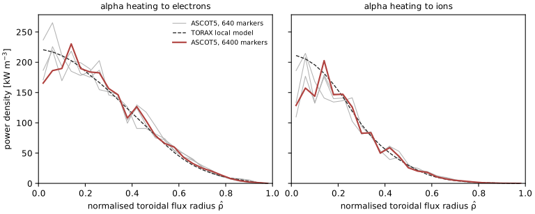
CSV: ascot_alpha_profile.csv. Provenance: profiles from tkit ascot-alpha at fcd8ce5 (job 2287778) and c8eaf6e (job 2286956); TORAX reference run iterhybrid_predictor_corrector at t = 5 s; figure script blog/figures/make_ascot_alpha_profile.py.

Results.

ASCOT5 production run vs TORAX’s local model, t = 5 s
total heating on TORAX’s cells	71.8 MW vs 70.5 MWC-064
radial position	centroid 0.370 vs 0.362, half-power radius 0.331 vs 0.325C-065
effect on TORAX after 2 s, heating held fixed	-0.009% in stored energy (central T_e +0.3%, T_e and T_i profiles 0.4% and 0.5%)C-067
orbit tolerance 10-8 vs 10-7, same markers	electrons -0.16%, ions +0.08%C-066

Birth power accounted for. The marker weights sum to AFSI’s birth rate to the last digit, so the markers’ birth power is the rate times their mean birth energy. That mean is 3.573 MeV, 1.5% above 3.52 MeVC-063. With the AFSI rate (+0.4% over TORAX’s) and the 3.52 against 3.5 MeV per alpha (+0.6%), it accounts for the whole 2.5% by which the birth power exceeds TORAX’s alpha power. The 1.3-1.4% “unexplained” excess of the first two jobs was the same quantity measured on 640 markers, whose mean birth energy scatters by ±0.012 MeV (±0.35%). Thermal motion of the reacting D and T raises the mean alpha energy above 3.52 MeV; whether that accounts for all of the 1.5% has not been computed (K-011 stays open until it has, and before ASCOT5 is used for neutral-beam ions).

Totals and shape. From birth power to TORAX’s cells: losses across the separatrix remove 0.7%, markers stopped at the thermal limit 0.8%, the energy books add 0.6%, and the interpolation onto TORAX’s cells 0.2%. The heating lies slightly further out than TORAX’s local model puts it, which deposits each alpha’s energy where it is born: the centroid and the half-power radius are larger in the production run and in each of the three 640-marker samples.

The core is not resolved cell by cell (K-012). Outside \(\hat\rho = 0.3\) every sample agrees with TORAX’s local model to 2-5% (NRMSD, normalised by the peak). Inside it, neighbouring cells of the production run differ by up to 21% (electrons) and 41% (ions), and its NRMSD from TORAX’s model there (13% for electrons, 20% for ions) is no smaller than the 640-marker samples’ (10-11% and 12-22%). If the scatter were sampling noise it would fall by about three with ten times the markers; it did not. Near the axis the equal-width \(\rho_\text{pol}\) bins hold little volume, which is the candidate cause; it has not been tested. Ion heating in the innermost cell is below TORAX’s local value in all four samples (110-186 kW/m³ against 211); electron heating is not consistently below. Neither is used: the totals, the electron/ion split and the shape moments are what M1 takes from ASCOT5.

Effect on TORAX. Held fixed from 5 s to 7 s, the production profiles change stored energy by -0.009% in stored energy (central T_e +0.3%, T_e and T_i profiles 0.4% and 0.5%)C-067, within the 640-marker result. The coupling-interval error of holding the heating fixed at all (-0.3% (central T_e -1.0%)C-047) is thirty times larger.

Correctness. tests/physics/test_ascot_alpha.py: the AFSI birth rate matches TORAX’s to 2%; markers carry the whole source with equal weights; the energy books close to 3% (markers stopped at 1.5 MeV); profiles handed to TORAX arrive cell by cell to 10^-12; a restart with held profiles keeps the alpha power fixed. tests/regression/test_cli_ascot_apply.py: the comparison reproduces TORAX’s totals and is exactly zero for identical profiles.

Design decisions.

• Equal marker weights, not a5py’s per-cell weights, so the source is complete at any marker count.
• The tolerance was set by a check, not by speed. The job reran a marker subset at a tighter tolerance; that check is what showed 10^-5 fails.
• Prescribed, not rescaled. Between updates the heating is held at ASCOT5’s profiles, not rescaled with TORAX’s fusion power, so the coupling error is measured directly (C-047).

Aurora: impurity transport

Aurora (MIT) models impurity transport and radiation. It builds and its Fortran core runs (smoke test); atomic data is not downloaded yet and it is not used by any run so far.

Changelog

• 2026-09-30: first published version (TORAX, FreeGSNKE, ASCOT5, Aurora).
• 2026-09-30: TORAX step energy and particle balance, and the pedestal pinning term (entry 8).
• 2026-10-01: ASCOT5 fusion-alpha heating, the orbit-tolerance check and the comparison with TORAX’s local model (entry 10).
• 2026-10-01: the RAPTOR L-mode benchmark from the TORAX paper, its discrepancy budget and time-step convergence; reverse-mode-only gradients through Newton (entry 11).
• 2026-10-01: second ASCOT5 job: orbit tolerance 10^-7, the per-marker time cap that stopped the production run, the energy-book overshoot reattributed to orbit tolerance (entry 12).
• 2026-10-02: third ASCOT5 job: the 6400-marker production run, the birth-power excess traced to the markers’ mean birth energy, the 10^-8 check, the unresolved core profile (K-012) (entry 15).